01.B - Hello Triangle
1 - Introduction
This tutorial builds on the previous one, so I highly recommend completing it before going through this tutorial if you have not done so already.
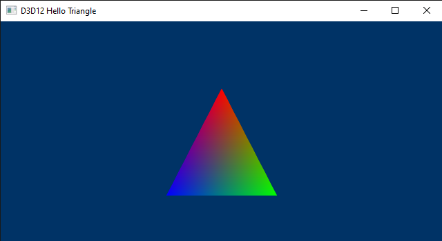
Here, we will examine the sample D3D12HelloTriangle, which draws a triangle on the render target. The related source code can be found in the official Microsoft repository (the link is provided at the end of the tutorial). Actually, the code of this sample hardly changes compared to that of D3D12HelloWindow. However, there is still a lot to explain. The reason is that this time we will make use of the rendering pipeline to draw something on the render target.
If you are familiar with video games, you know that the image you see on the screen is only a 2D representation of 3D geometries composed of polygons (most of the time triangles) defined by vertex locations in 3D space.
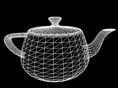
It can be stated that the whole art of computer graphics boils down to creating a 2D representation from a 3D scene. Indeed, this is the result of processing 3D geometries through a rendering pipeline, which will be briefly discussed in the next section.
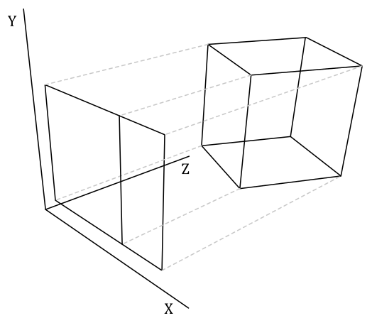
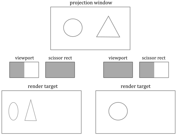
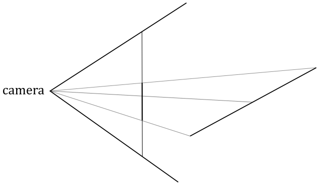
In the image below, you can see a 3D scene projected onto a 2D rectangle\window lying on a plane in front of a special viewpoint called the camera. You can think of a 2D projection window as the film of a camera (or the retina of the human eye) that captures the light and allows the creation of a 2D representation from a 3D scene. Eventually, this 2D representation is mapped to the render target, which, in turn, is mapped to the window’s client area.
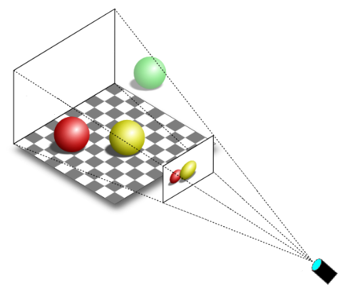
You can easily guess that only a particular region of the 3D scene should be captured by the camera (that is, we generally won’t capture the whole 3D scene). The extent of the region captured can be controlled in a similar way to how we set the field of view (FOV) of the camera lens when we want to take a picture. However, in computer graphics, the film is typically positioned in front of the camera lens, not behind.
Now, we need to define a couple of terms that we will use throughout the rest of this tutorial:
Monitors are raster displays, which means the screen can be seen as a two-dimensional grid of small dots called pixels. Each pixel displays a color that is independent of other pixels. When we render a triangle on the screen, we don’t actually render a triangle as one entity. Instead, we illuminate the group of pixels that are covered by the triangle’s area.
Textures are typically 2D digital images composed of small dots called texels that contain various information (e.g., color, distance, direction, etc.). We can also use textures as render targets, essentially treating them like a canvas where we can draw by setting colors to texels. Subsequently, the final image representing a frame, can be mapped to the window’s client area to display the result to the user.
[!NOTE]
A physical pixel is a square with an area, but its coordinates refer to a specific point (usually, the top-left corner of the pixel). However, GPU calculations and sampling operations often occur at the center of the pixels. When we describe a monitor as a 2D grid of dots, we are actually referring to rows and columns intersecting at pixel coordinates. The same considerations also apply to textures, which can be seen as grids of texels (texture elements) with an area, whose coordinates refer to a specific point within the texel’s area. We will revisit this concept in an upcoming tutorial.
In the next section, we will briefly discuss what a graphics pipeline is and how it can be used to draw on a render target.
2 - Direct3D rendering pipeline overview
GPUs are equipped with thousands of programmable cores, which means that they can execute programs in the form of instructions provided by a programmer, much like how CPU cores run C++ applications. As illustrated below, CPUs typically have fewer cores than GPUs. However, GPU cores are smaller and more specialized in processing tasks that can be divided up and processed across many cores. In particular, GPUs use parallelism to execute the same instructions on multiple cores simultaneously, resulting in high-speed processing of vast amounts of data. On the other hand, CPUs excel at executing many sequential instructions on each core to execute multiple tasks on small data really fast.
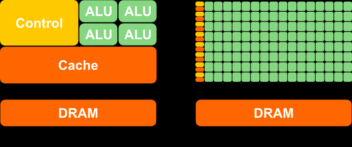
CPU (on the left) versus GPU (on the right)
GPUs that support Direct3D can execute programs on their cores to perform the work of various stages composing a pipeline. Direct3D provides different pipeline types, but we will focus on the rendering pipeline (also called the graphics pipeline) for now. A rendering pipeline defines the steps needed to draw something on the render target. In particular, the following image illustrates the stages of the rendering pipeline used to draw on a render target with the Direct3D API.
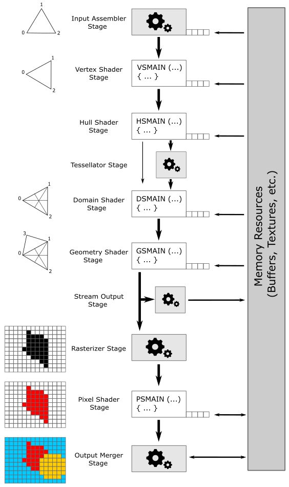
Programmable stages can execute programs (often called shader programs, or simply shaders, with the GPU cores executing them often referred to as shader cores) written by programmers. Configurable stages (the rectangles with gear wheels in the above illustration) can’t be programmed: they always execute the same code, but you can still configure their state. This means you can’t specify what a configurable stage can do, but you can still specify how it performs its task. For this reason, they are often called fixed-function stages.
Data flows from input to output through each of the configurable or programmable stages. In other words, each stage consumes the input from the previous stage and provides its output to the next one (which can use it as input).
-
Input-Assembler Stage - The input assembler is responsible for supplying data to the pipeline. This stage takes its input from user-filled buffers in memory that contain arrays of vertices (and often also indices), and from those buffers it assembles primitives (triangles, lines and points) with attached system-generated values (such as a primitive ID, an instance ID, or a vertex ID) to pass to the next stage, vertex by vertex.
-
Vertex Shader Stage - The vertex shader processes vertices from the input assembler. It usually performs operations such as transformations, skinning, and per-vertex lighting. A vertex shader always takes one vertex as input and return one vertex as output. So, a vertex shader needs to run multiple times to process all the vertices of the primitives assembled by the input assembler.
-
Hull Shader Stage - The hull shader operates once per patch. A patch is a set of control points whose interpolation defines a piece of curve or surface. You can use this stage with patches from the input assembler. The hull shader can transform input control points into output control points. Also, it can perform other setup for the fixed-function tessellator stage. For example, the hull shader can output tess factors, which are numbers that indicate how much to tessellate, which refers to the primitive density in the surface or curve described by the output patch.
-
Tessellator Stage - The tessellator is a fixed-function unit whose operation is defined by declarations in the hull shader. That is, the tessellator operates once per patch that is output by the hull shader. The purpose of the tessellator stage is to sample the domain (quad, tri, or line) of the patch by tessellating it. Also, the tess factors generated by the hull shader notify the tessellator how much to tessellate (that is, dividing a geometric shape into smaller, connected primitives) over the domain of the patch.
-
Domain Shader Stage - The domain shader is invoked once per sample (generated by the tessellator). Each invocation is identified by the coordinates of the sample over the domain of the patch, as well as the output control points produced by the hull shader. The role of the domain shader is to turn the sample coordinates into something tangible (such as, a vertex position in 3D space), which can be sent down the pipeline for further processing.
-
Geometry Shader Stage - The geometry shader processes entire primitives. That is, its input can be three vertices for a triangle, two vertices for a line, or a single vertex for a point. The geometry shader supports limited geometry amplification and de-amplification. Given an input primitive, the geometry shader can discard the primitive, or emit one or more new primitives.
-
Stream Output Stage - The stream output is designed for streaming primitive data from the pipeline to memory on its way to the rasterizer. Data can be streamed out and/or passed into the rasterizer. Data streamed out to memory can be recirculated back into the pipeline as input data for the input assembler or read-back from the CPU.
-
Rasterizer Stage - The rasterizer converts primitives into a raster images (composed of pixels that need to be processed by subsequent stages to be rendered on the screen). It also takes into account the viewport and scissor rectangles (more on this later). As part of the rasterization process, the per-vertex attributes are interpolated to calculate the per-pixel attributes across each primitive (a vertex is essentially a collection of attributes). Additionally, the rasterizer takes into account the viewport and scissor rectangles when performing its task. Further details will be provided in later sections of this tutorial.
-
Pixel Shader Stage - The pixel shader receives interpolated attributes for every pixel of a rasterized primitive generated by the rasterizer and returns per-pixel data (such as color), such as a color, that can be possibly stored as a texel in the render target; it depends on the last stage of the pipeline. The pixel shader allows to enable sophisticated shading techniques, including per-pixel lighting and post-processing, to enhance the overall visual quality of the rendered image.
-
Output-Merger Stage - The output merger (OM) stage is the final step for determining which pixels are visible, through depth-stencil testing, and how to eventually blend them with the corresponding texels in the render target. In particular, it is responsible for combining various types of output data (pixel shader returned values, depth, stencil and blend information) with the contents of the render target and depth/stencil buffer to generate the final pipeline result (the final image we want to draw on the render target before showing it on the screen).
[!NOTE]
Hull Shader, Tessellator and Domain Shader together form the Tessellation stage. They are optional and we won’t use them for a while. The same goes for the Geometry Shader and the Stream Output stage.
As illustrated in the image above, many stages can take part of their input by reading resources from GPU memory (in addition to the input passed from the previous stage), and some of them can write their output in GPU memory as well. The little squares at the bottom right of some stages represent the slots where descriptors\views are bound. At the left of each stage, you can find a visual description of the task usually performed by the stage. VSMAIN, PSMAIN, etc., suggest that programmable stages execute shader programs.
[!NOTE]
A descriptor (or view) is a data structure that fully describes a resource to the GPU (type, dimension, GPU virtual address, and other hardware-specific information). This means the size of a descriptor can change from GPU to GPU. Usually, descriptors are bound to the slots of the stages, rather than the actual resources. This way, the GPU can access resources by reading the descriptors bound to the slots used in the shader program being executed.
[!IMPORTANT]
Binding slots are not physical blocks of memory or registers that a GPU can access to read descriptors. They are simple names (character strings) used to associate descriptors to resource declarations in shader programs. However, since the documentation uses the term “slots” in the context of resource binding, I still opted to represent them in the illustration above as physical blocks. As described in the previous tutorial, descriptors are stored in a descriptor heap. In the remainder of this tutorial we will see how a GPU accesses descriptors during the execution of a shader program.
[!NOTE]
Even though the documentation does not explicitly distinguish between descriptors and views, it is sometimes helpful to visualize a descriptor as the physical block of memory where to store a view, which can be perceived as an instance of a hardware-specific type (structure) that encapsulates information about a resource.
The depth buffer is a texture associated with the render target (both should be the same size). The depth buffer is used to store depth information that informs us how deep each visible pixel is in the scene. When Direct3D renders 3D primitives to a render target, the output merger stage can use the depth buffer to determine how the pixels of rasterized polygons occlude one another.
Typically, the stencil buffer is coupled with the depth buffer (that is, both share the same buffer in memory, though using different bits) and stores stencil information to mask pixels. The mask controls whether a pixel is drawn or not on the render target, enabling the creation of specialized effects such as dissolves, decaling, and outlining. We will return to the stencil buffer in a later tutorial.
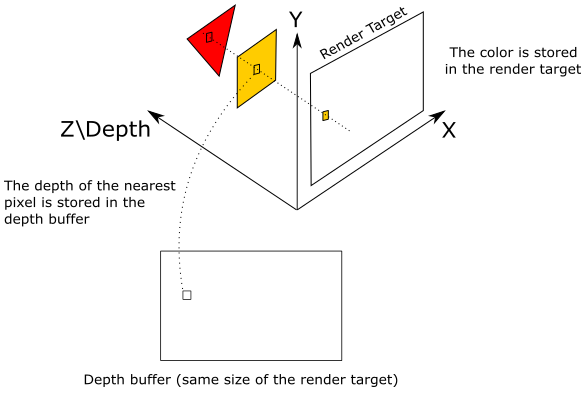
In the image above, the 2D projection window lies in the plane identified by the X- and Y-axes. We already know that the projection window is eventually mapped to the render target, so let’s temporarily assume that we are directly drawing on the render target (without passing through the projection window). The Z-axis is used to measure the depth of the pixels (that is, their distance from the XY-plane). As you can see, the texel of the render target will store the pixel color of the yellow square, which occludes the pixel of the red triangle. Indeed, the value stored in the corresponding texel of the depth buffer (that is, at the same position of the texel in the render target) is the depth of the nearest pixel: the one of the yellow square, in this example. So, the pixel of the triangle will be discarded if the depth test is enabled. On the other hand, if the depth test is disabled, the texel of the render target will store the color of the last pixel processed by the pixel shader since it will always overwrite whatever color is stored in that texel. Observe that if blending is enabled, the pixel color is blended with the color stored in the corresponding texel of the render rather than overwriting it.
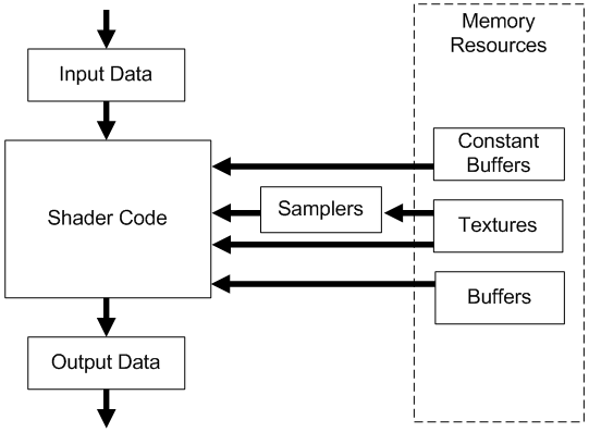
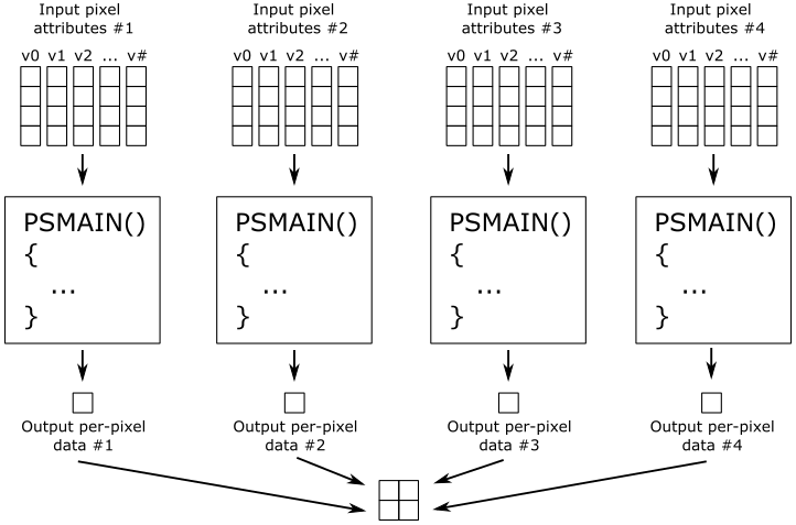
The following image shows how a generic programmable stage works.
-
Input Data: A vertex shader receives its input from the input assembler stage; geometry and pixel shaders receive their inputs from the previous stage. This data typically consists of multiple values, called attributes, that describe various aspects of the geometric data being processed. For example, attributes might include the position or color associated with a vertex, or the texture coordinates for a pixel. Additional inputs include system-value semantics, which are consumable by the first stage in the pipeline to which they are applicable.
-
Output Data: A shader generate output results to be passed on to the subsequent stage of the pipeline. For a geometry shader, the amount of data output from a single invocation can vary. Semantics also apply to elements of the output data to convey information about the intended use to the next stage. Semantics are required for all elements passed between shader stages.
-
Shader Code: GPUs can read from memory, perform vector floating point and integer arithmetic operations, or flow control operations. We write shader programs in HLSL (High Level Shader Language), a procedural language similar to C, to instruct the GPU on the operations to execute.
-
Samplers: Samplers define how to sample and filter textures.
-
Textures: Textures can be filtered using samplers, or read on a per-texel basis directly with the Load intrinsic function.
-
Buffers: A buffer is a collection of fully typed data grouped into elements (just like an array). Buffers are never filtered, but can be read from memory on a per-element basis.
-
Constant Buffers: Constant buffers are optimized for shader constant-variables. They are designed for more frequent update from the CPU; therefore, they have additional size, layout, and access restrictions.
[!NOTE]
I know! I should elaborate further on semantics. In general, data passed between pipeline stages is completely generic. A semantic is a textual name we can associate to every element in the input data to establish its intended use. You can associate arbitrary strings with no special meaning to elements of the input data as semantics. However, there are several predefined semantics with specific meanings when attached to elements of the input data. For example, POSITION and COLOR, which are pretty self explanatory. A system-value semantic is simply a semantic that start with “SV_”, and that can be associated with additional data generated and\or consumed by the stages of the pipeline to pass and\or identify info in the input data with a special meaning. For example, pixel shaders can only write to elements associated with the SV_depth and SV_Target system-value semantics. Don’t worry if it’s not entirely clear at the moment. It’s simpler than it may seem, and practical examples will be provided later in the tutorial, specifically in the final part when we examine the code of the sample.
This section provided only a brief overview of the rendering pipeline, so if this is your first encounter with these concepts, a bit of confusion is completely normal. However, dont worry! We will revisit each of these topics in the following sections and upcoming tutorials to provide detailed explanations.
3 - Resources management
In DirectX, we can create several types of resources through the device object (that is, through a pointer to the ID3D12Device interface). While the initial tutorial covered creating a command queue, a command allocator, and a command list, we can also produce different types of buffers (constant, typed, structured, raw) and textures (1D, 2D, 3D), or even arrays of these resources.
Typically, we call the ID3D12Device::CreateCommittedResource method whenever we want to create a buffer or a texture. The arguments passed to CreateCommittedResource specify where to allocate memory space, the type of resource to create, its initial state, and a pointer to a memory block that will receive the interface pointer to the created resource for referencing it within our application. With CreateCommittedResource we can also create typeless resources if format information is missing. However, when you want the GPU to access a typeless resource, you need to bind a view that fully describes it; otherwise, the GPU might have no idea how to access it.
3.1 - Memory
GPUs have access to four types of memory:
-
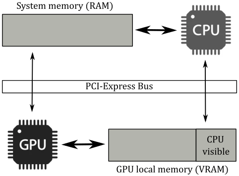
Dedicated video memory: this is memory reserved\local to the GPU (VRAM). It’s where we allocate most of the resources accessed by the GPU (through the shader programs).
-
Dedicated system memory: it is a part of the dedicated video memory. It’s allocated at boot time and used by the GPU for internal purposes. That is, we can’t use it to allocate memory from our application.
-
Shared system memory: this is CPU-visible GPU memory. Usually, it is a small part of the GPU local memory (VRAM) accessible by the CPU through the PCI-e bus, but the GPU can also use CPU system memory (RAM) as GPU memory if needed. Shared system memory is often used as a source in copy operations from shared to dedicated memory (that is, from CPU-accessible memory to GPU local memory) to prevent the GPU from accessing resources in memory via the PCI-e bus. It’s write-combine memory from the CPU point of view, which means that write operations are buffered up and executed in groups when the buffer is full, or when important events occur. This allows to speed up write operations, but read ones should be avoided as write-combine memory is uncached. This means that if you try to read this memory from your CPU application, the buffer that holds the write operations need to be flushed first, which makes reads from write-combine memory slow.
-
CPU system memory: it’s system memory (RAM) that, like shared system memory, can be accessed from both CPU and GPU. However, CPUs can read from this memory without problems as it is cached. On the other hand, GPUs need to access this memory through the PCI-e bus, which can be a bottleneck compared to the direct memory access of CPUs through the system memory bus.
[!NOTE]
If you have an integrated graphics card or use a software adapter, there is no distinction between the four memory types mentioned above. In that case, both the CPU and GPU will share the only memory type available: system memory (RAM). This implies that your GPU may have limited and slower memory access.
When the CreateCommittedResource function is invoked, we need to specify the type of memory where space should be allocated for the resource we want to create. You can indicate this information in two ways: abstract and custom. In the abstract way, we have three types of memory heaps that allow abstraction from the current hardware.
-
Default heap: memory that resides in dedicated video memory.
-
Upload heap: memory that resides in shared video memory.
-
Readback heap: memory that resides in CPU system memory.
Therefore, using the abstract approach, regardless of whether you have a discrete GPU (that is, a dedicated graphics card) or an integrated one, physical memory allocations are hidden from the programmer.
On the other hand, if you want different allocations based on the type of hardware, you can explore the custom way, which allows you to specify the caching properties and the memory pool where you want to allocate space. However, we won’t delve into the details here, as we will mostly use the abstract way to allocate both CPU-visible and GPU-visible memory in the upcoming tutorials.
A resource is considered resident in memory when it is accessible by the GPU. Typically, when you create a resource with CreateCommittedResource, you allocate an amount of GPU-visible memory large enough to contain the resource. At that point, the resource is resident in memory and remains so until it is destroyed (or explicitly evicted from memory).
3.2 - Views and descriptors
As mentioned earlier, a resource can be created in a generic format, and a view is an instance of a hardware-specific type that can be bound to the rendering pipeline to fully describe a resource to the GPU. In other words, we use views to bind resources to resource declarations in shader programs (more on this later). We can create a view to a resource with one of the Create*View methods. Each of these methods creates a view to a resource from the information passed as an argument, and stores the view in the descriptor passed in the last parameter (as a CPU descriptor handle). Remember that descriptor heaps must be CPU visible because we need to store views in descriptors.
Since views hold hardware-specific information for different resource types, the size of a view depends both on the hardware and the type of resource described. In the first tutorial, we have seen that to access descriptors in a descriptor heap, we offset CPU or GPU descriptor handle values. This means that not all descriptors can share the same descriptor heap. Also, not all views can be stored in descriptors and must be used directly in copy operations (more on this shortly). Below is a list of all views we can create.
- Constant buffer view (CBV)
- Unordered access view (UAV)
- Shader resource view (SRV)
- Samplers
- Render Target View (RTV)
- Depth Stencil View (DSV)
- Index Buffer View (IBV)
- Vertex Buffer View (VBV)
- Stream Output View (SOV)
CBVs are used to describe constant buffers, SRVs are used to describe read-only textures and buffers, and UAVs are used to describe textures and buffers when both read and write access from multiple threads is needed.
Samplers are not exactly views (you can think of them as self-contained objects). However, samplers are considered views because they are often managed in a similar way (more on this shortly).
We have already encountered RTVs in the first tutorial. DSVs are used to describe depth-stencil buffers.
IBVs and VBVs are used to describe index and vertex buffers, respectively.
SOVs are used to describe stream output buffers (we will cover them in a later tutorial).
[!NOTE]
CBVs, SRVs, and UAVs are of the same size, allowing them to share the same descriptor heap.
CBVs, SRVs, UAVs, and samplers can be stored in descriptor heaps allocated in write-combined memory (possibly on CPU-visible GPU local memory) by setting D3D12_DESCRIPTOR_HEAP_FLAG_SHADER_VISIBLE as a flag in the D3D12_DESCRIPTOR_HEAP_DESC structure passed as an argument to the CreateDescriptorHeap function. In this case, we refer to them as shader-visible descriptor heaps, indicating that the GPU needs to access their descriptors. However, samplers cannot share a descriptor heap with CBVs, SRVs, and UAVs, as they require a dedicated descriptor heap.
On the other hand, RTVs and DSVs must be stored in descriptor heaps allocated in CPU system memory by specifying D3D12_DESCRIPTOR_HEAP_FLAG_NONE as a flag in D3D12_DESCRIPTOR_HEAP_DESC. That’s why we call them non-shader-visible descriptor heaps to specify that the GPU doesn’t need to access their descriptors (as mentioned in the first tutorial, RTVs are copied in the command list, and the same applies to DSVs). Both RTVs and DSVs need a separate descriptor heap from all other views. CBVs, SRVs, and UAVs can also be stored in non-shader-visible heaps.
IBVs, VBVs, and SOVs don’t need to be stored in a descriptor (similarly to descriptors directly provided as root arguments, which will be described in more detail later). These descriptors, like RTVs and DSVs, are directly recorded into (copied to) the command list.
3.3 - Transitions
Consider a scenario where a command list includes command to both read and write to a resource. While a GPU can execute commands in parallel, it should not start reading the texture until all ongoing write operations have completed to avoid data races.
In Direct3D 12, we specify the intended use of a resource by transitioning its state. For example, if the GPU is to read a texture, that texture must be in a readable state. The programmer is responsible for recording transition barriers in the command list to inform the GPU about the intended usage of each resource, enabling it to determine which operations can be executed concurrently and which cannot.
In Direct3D 12, most per-resource state is managed by our application with ID3D12GraphicsCommandList::ResourceBarrier. At any given time, a resource is in exactly one state, determined by the D3D12_RESOURCE_STATES flag provided to the ResourceBarrier function.
3.4 - Root signature
Obviously, GPUs need a way to access resources stored in GPU heaps (default, upload or readback) from shader programs. For example, in HLSL (the language used to write shader programs) you can declare the following variable:
Texture2D g_texture : register(t0);
It may seem that g_texture is a variable that represents a 2D texture. That’s not entirely wrong, but we can be more precise. The Microsoft documentation states that resources declared in HLSL are bound to virtual registers within logical register spaces:
t – for shader resource views (SRV)
s – for samplers
u – for unordered access views (UAV)
b – for constant buffer views (CBV)
The register attribute specifies that g_texture is bound to slot (virtual register) $0$ of the register space t, which is reserved for SRVs. Therefore, this variable allows access to a descriptor that holds an SRV describing a 2D texture. The use of the term “register” is a bit misleading in this case. There are no registers or memory regions behind binding slots. A more appropriate term would have been linkname, indicating that a slot name is only used to link descriptors in memory and resource declarations in HLSL. In this case, we are using the string t0 to bind a descriptor stored in a GPU heap (maybe included in a descriptor heap or in a command list) to a resource declaration in a shader program.
That said, the following illustration shows the general idea: we can bind descriptors in memory to variables declared in the shader code by associating both a root signature and a shader-visible descriptor heap with the command list. Now, we are elaborating further on this general idea.
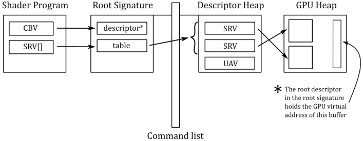
Once the resources and their corresponding descriptors have been created (on the CPU timeline), we can associate a structure called root signature to the command list. The root signature acts like a function signature in C\C++: it describes the types of the input and output parameters. In other words, the root signature defines the data types that the shader programs of all programmable stages should expect both as input and output data through the resource variables declared in the HLSL code (that is, what they need to read and\or write). More specifically, a root signature is an array of root parameters that describe the types of descriptors we wish to bind to the pipeline (or rather, to the resource variables declared in the shader code of the programmable stages of the pipeline), along with the corresponding binding slots (virtual registers), so that it is possible to associate root parameters with variables in HLSL.
[!NOTE]
Similar to a function signature, a root signature only describes the types of the descriptors. The actual descriptors need to be passed as root arguments to the root parameters by recording specific commands (dedicated to this purpose) in the command list.
There are three types of root parameters:
-
Root constants: 32-bit constants inlined in the root arguments. The size of each root constant in the root signature is 1 DWORD.
-
Root descriptors: descriptors inlined in the root arguments. Mainly used for descriptors that are frequently accessed and that specifically describes buffers (i.e., not textures). The size of each root descriptor in the root signature is 2 DWORD.
-
Root descriptor tables (also called descriptor tables, or root tables): pointers to a set of contiguous descriptors in a shader-visible descriptor heap associated with the command list. The size of each root descriptor table in the root signature is 1 DWORD.
[!NOTE]
Root constants show up as a constant buffer in the shader programs. This means you still have to define the corresponding type\structure in the shader code (refer to the next note). However, using root constants, you don’t need to create a constant buffer and the related view to be bound to the pipeline, as the constant buffer data is passed to the GPU directly in the root argument. We will return to root constants in a later tutorial.
[!NOTE]
Root descriptors are not really descriptors. They only take 2 DWORD to store the GPU virtual address of the corresponding resource. That’s why you can only use them for buffers: GPUs need more information to access textures (size, type, format, etc.). As we will see in an upcoming tutorial, if a buffer holds one or more elements of a user defined type, this needs to be fully defined in the HLSL code, so a GPU can access them by only knowing the starting address of the buffer. However, it’s up to the programmer to not access the buffer out of bounds.
[!NOTE]
Root tables are convenient when you want to bind sets of descriptors to arrays of resources declared in HLSL. A root table just stores a 32-bit value (1 DWORD) representing the byte offset of a set of contiguous descriptors from the start of a shader-visible descriptor heap associated with the command list. Also, a root table allows to bind different types of descriptors, provided that they are contiguous in a descriptor heap.
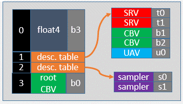
The figure below is an example of a simple root signature. The root parameter at index 0 is a collection of four root constants (as float4 is a structure of four float of 1 DWORD each). The root parameter at index 3 is a root descriptor that holds the GPU virtual address of a resource in a GPU heap. The root parameters with indices 1 and 2 are root descriptor tables. As you can see, the descriptor table at index 1 is a set of five contiguous descriptors divided into three ranges of descriptors with different types (2 SRVs, 2 CBVs, and 1 UAV). When we pass a root argument by recording the dedicated command in a command list, we must also specify the index of the corresponding root parameter.
[!NOTE]
Binding slots are specified both for root constants and root descriptors. However, for root tables, they are specified at a range level. Additional information will be provided in an upcoming tutorial, when we cover root tables in more detail.
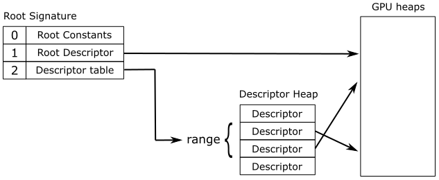
In the figure below, you can see that for root constants, there is no indirection. This means that the shaders can read the values directly from the root arguments passed at command list recording time. For root descriptors, there is a level of indirection, since they contain GPU virtual addresses to resources in GPU heaps. Lastly, with root descriptor tables, there is a double level of indirection, as they hold offsets to descriptors, which in turn hold GPU virtual addresses to resources.
[!NOTE]
Obviously, increasing the levels of indirection leads to increased complexity (i.e., longer time to access resources). However, it also allows for the efficient management of a larger set of descriptors with different types.
Static samplers deserve special mention as they are part of a root signature, but separated from the root parameters. Therefore, they do not have any cost in the size of a root signature. The management of static samplers is implementation-specific. However, some GPUs implicitly store static samplers in a descriptor heap hidden in reserved space, and automatically bind them to the related declarations in the shader code. This is why samplers are considered like other views. There are no downsides to taking advantage of the convenience of static samplers, so use them whenever possible, as you don’t need to explicitly create descriptor heaps and views.
We must associate a root signature with a command list in order to set up a parameter space where root arguments can be mapped. As noted above, root arguments are passed to root parameters by recording dedicated commands in the command list. When the GPU executes these commands, the root arguments are stored in a root argument space, a memory region near the GPU core registers, so that a GPU can quickly reference them during the execution of a shader program. However, this fast memory region is limited in size. Fortunately, most GPUs can also spill to slower memory regions whenever the fast one is full.
[!NOTE]
If you pass a root argument for a root parameter to draw an object A and then, in the same command list, you pass a different root argument for the same root parameter to draw an object B, the driver may need to copy the whole memory region where the root arguments are stored. However, if the root arguments are split into fast and slow memory regions, the driver can only copy the region of memory where the new root arguments reside. This allows to execute drawing commands in parallel, where each draw references the proper memory region of root arguments.
[!IMPORTANT]
The maximum size of a root signature is 64 DWORDs. However, this is more a suggestion (rather than a rule) to keep in mind that smaller root signatures allow for the root arguments to be stored exclusively in the fast memory region. The documentation also recommends sorting root parameters (within the root signature) from most frequently changing to least frequently changing. In other words, root parameters that receive different root arguments within the same command list should be placed before root parameters that remain static. This approach provides the driver with a better chance of only copying root arguments from the fast memory region (which is more efficient).
[!IMPORTANT]
Changing the root signature associated with a command list is relatively inexpensive. However, this invalidates the current root arguments, which require re-setting. Unfortunately, this final operation is more expensive, so minimize the number of root signature changes.
Changing a shader-visible descriptor heap associated with a command list can be expensive, as the GPU must first execute all the pending work that depends on the currently bound shader-visible descriptor heap. Therefore, whenever possible, set a shader-visible descriptor heap once, after creating the command list.
3.4.1 - Root signature version
Microsoft continuously updates the design of the root signature to enable more hardware optimizations by the drivers.
Root Signature version 1.0 allows descriptors in a descriptor heap, and\or resources they point at, to be freely changed by applications any time that command lists referencing them are in flight on the GPU. However, this flexibility in changing descriptors and the related resources is paid for with a poor optimization.
Root version 1.1 lets drivers produce more efficient memory accesses by shaders if they know the promises an application can make about the static nature of descriptors and resources they point to during command list recording and execution. For example, drivers could remove a level of indirection for accessing a descriptor in a heap by converting a descriptor table into a root descriptor if both the descriptor table and the resource it points to are found to be static.
We can make promises about the static nature of descriptors (in a descriptor heap) and/or data they point to by setting some flags during the creation of the related root descriptor tables.
Unless otherwise indicated (that is, if no flag is specified), using root signature version 1.1 will set descriptors to be static by default.
As for the data they point to, it depends on the type of descriptor. CBVs and SRVs data are DATA_STATIC_WHILE_SET_AT_EXECUTE by default, which means the driver assumes that the resource pointed to by a descriptor can change up until the command list starts executing and stays unchanged for the rest of the execution. UAVs data are DATA_VOLATILE by default, which means the driver assumes the resources pointed to by a descriptor to be editable both during command list recording and execution.
You can explicitly set a descriptor to DESCRIPTORS_VOLATILE, which means the driver assumes descriptors can change during command list recording and stay unchanged for the rest of the execution. DESCRIPTORS_VOLATILE and DATA_VOLATILE are the only supported behaviors of Root Signature version 1.0. That’s why the driver can’t make assumptions about the static nature of descriptors and data.
4 - The Pipeline State
The pipeline state defines the behavior\setup of every stage in the pipeline when we are going to draw something. We can set the state of both configurable and programmable stages in a single object called the pipeline state object (PSO), which describes most of the state of the pipeline. A PSO is a unified pipeline state object that is immutable after creation (you have to create a new one to define a different pipeline state). A quick summary of the states that can be set in a PSO includes:
-
The bytecode for all shader programs (that defines the states of programmable stages).
-
The input vertex format.
-
The primitive topology type (point, line, triangle, patch).
-
The blend state, rasterizer state and depth stencil state.
-
The depth stencil and render target formats, as well as the render target count.
-
Multi-sampling parameters.
-
A streaming output buffer.
-
The root signature.
We will cover each of these points both later and in upcoming tutorials.
As mentioned earlier, while most of the pipeline state is configured using a PSO, certain parameters need to be set directly in the command list. The following list highlights the states that must be configured directly in a command list.
-
Resource bindings (vertex and index buffers, render target, depth-stencil buffer, descriptor heaps).
-
Viewport and Scissor rectangles.
-
Blend factors.
-
The depth stencil reference value.
-
The input-assembler primitive topology order and adjacency type (line list, line strip, line strip with adjacency data, etc.).
As for the first point, recall that IBVs, VBVs, RTVs, and DSVs are copied into the command list. Furthermore, we can associate a shader-visible descriptor heap to a command list. We will revisit the remaining points in both this tutorial and upcoming ones.
To set the part of the pipeline state defined within a PSO, we record a dedicated command in the command list with ID3D12GraphicsCommandList::SetPipelineState. Alternatively, we can set the same state during the creation or reset of a command list with ID3D12Device::CreateCommandList and ID3D12GraphicsCommandList::Reset, respectively. The result is the same: a command (in the command list) that sets the pipeline state. Either way, we pass a PSO as an argument. If no PSO is specified in CreateCommandList, a default initial state is used. Then, we can use SetPipelineState to change the PSO associated to the command list.
Therefore, all of the pipeline state is recorded in a command list, and none of the pipeline state that was set by previously executed command lists will be inherited. Additional information on pipeline state inheritance will be provided in the next tutorial.
The documentation states that, ideally, the same root signature should be shared by more than one PSO whenever possible. This implies that we should design the root signature to be as general as possible. The last sentence suggests that root signatures could easily become large structures, seemingly in contrast with the earlier emphasis on the need for small root signatures. However, the key is always to find the right balance for the specific application on which we are working.
We set both a PSO and a root signature in the command list so that the GPU can use them to define (most of) the pipeline state and the types of resources to bind to the pipeline (recall that non-PSO states are individually set in the command list). For binding purposes, we may also need to set a couple of shader-visible descriptor heaps to the command list – one for CBVs\SRVs\UAVs and another for dynamic samplers, since samplers cannot share a descriptor heap with other views. This setup allows us to bind sets of descriptors in a descriptor heap through root descriptor tables in the root signature.
When recording a drawing command in a command list, it’s important that the root signature stored in the PSO associated with (recorded in) the command list matches the one directly associated with the command list. Failure to do so results in undefined behavior. As emphasized earlier, root signatures should be kept as small as possible while still being large enough to be shared by multiple PSOs. This enables switching between PSOs without changing the root signature associated with the command list, which would otherwise invalidate the root arguments.
We create a PSO with ID3D12Device::CreateGraphicsPipelineState, which requires a D3D12_GRAPHICS_PIPELINE_STATE_DESC as a parameter. This structure describes a pipeline state object, meaning that we need to set its fields to define the part of pipeline state within a PSO, such as bytecode of the shaders, root signature, and so on. When we call CreateGraphicsPipelineState to create a PSO, the driver compiles the bytecode in machine code executable by the GPU. The driver also uses the root signature inside the PSO to embed the traversal details in the machine code to let the GPU know how to access resources (through the root arguments specified in the command list).
[!NOTE] While we won’t delve into the driver’s implementation-specific details regarding the translation of bytecode to GPU machine code, we can shed some light on the traversal details embedded in the machine code.
Regarding root constants, a plausible implementation might involve loading them directly into registers, allowing the GPU to access the associated values without any additional memory reads during shader execution.
For root descriptors, an implementation could specify loading GPU virtual addresses for the corresponding resources into registers. In this case, the GPU would need to read from memory to access them, introducing a level of indirection.
In the case of root tables, an implementation might load the address of the currently bound shader-visible descriptor heap into one register and the byte offset of a set of descriptors into another register. This would require the GPU to read from memory twice – once to obtain a descriptor and a second time to access the related resource, resulting in two levels of indirection.
At first glance, one might assume that root constants would always be the optimal choice. Unfortunately, GPUs have a limited number of registers, and if you use an excessive number of root constants, the driver might need to spill them to memory, effectively introducing a level of indirection.
At this point, you might question the necessity of specifying the root signature twice — both in the PSO and the command list. In simpler terms, if the root signature in the PSO and the command list must match, couldn’t the command list simply retrieve this information from the associated PSO? The key distinction lies in the purpose of the root signature in each context. The PSO uses the root signature only for compiling the bytecode, while a command list uses the root signature to establish the parameter space, enabling the mapping of root arguments to root parameters. Furthermore, we might set root arguments before binding a PSO to a command list. Consequently, the parameter space must be configured even in the absence of a PSO.
Once more, don’t be concerned if things seem a bit unclear right now. The upcoming four sections will delve deeply into the pipeline stages used by the sample discussed in this tutorial (D3D12HelloTriangle) to render a triangle on the target. Additionally, in the final section, we’ll review the sample’s source code, offering a practical application of the theoretical concepts discussed thus far. By the end of this tutorial, you’ll have a foundational understanding of the rendering pipeline and how to use it for rendering on the target.
5 - The Input Assembler
The input assembler is the first stage of the rendering pipeline. It assembles primitives (points, lines, triangles) from a couple of user-defined arrays (known as vertex and index buffers) and passes those primitives to the vertex shader, vertex by vertex. It’s a fixed-function stage, so we can only set up its state. In particular, we need to bind at least an array of vertices (the vertex buffer) and, optionally, an array of indices (the index buffer) that describe, primitive by primitive, one or more meshes we want to render. As we’ll explore in this section, the input assembler requires additional information to execute its task effectively.
[!NOTE]
The input assembler doesn’t actually assemble primitives from the vertex buffer. It simply passes vertex data to the vertex shader in a specific order, determined by the input assembler state, which is stored both in the PSO and directly in the command list (more on this will be discussed shortly). As a result, the vertex shader will receive and process, one by one, the vertices of each primitive described in the vertex buffer, in the specific order designated by the input assembler. However, remember that GPUs can run the vertex shaders for vertices of multiple primitives simultaneously in parallel.
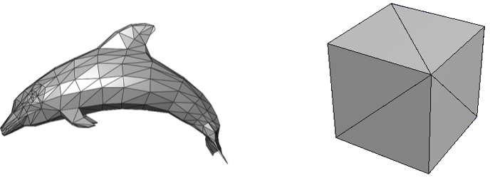
5.1 - Meshes
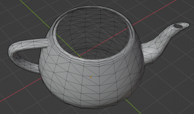
A mesh is a geometrical structure composed of polygons\primitives (often triangles) which are defined by their vertices. Regardless of whether it is a complex model made with graphic modeling tools such as 3ds Max or Blender, or a straightforward cube created programmatically, the underlying structure used to represent it in memory is the same: an array of vertices (known as the vertex buffer) that describes, vertex by vertex, the primitives that compose the mesh. Therefore, it is useful to understand what vertices are and how they can be organized in memory as a vertex buffer.
5.2 - Vertex buffer
When you think of a vertex, position is the first thing that comes to mind. However, in the context of computer graphics, a vertex is more like a structure whose fields describe some important attributes of the vertex such as position, color, and so on. A vertex buffer is simply a buffer that contains an array (that is, a contiguous collection) of vertices.
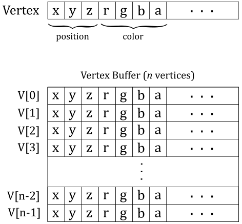
Unfortunately, the vertex buffer illustrated in the image above only represents the logical representation from our point of view, which reflects how we expect the input assembler to interpret the vertex buffer. Indeed, if we were to bind an array of vertices without providing additional information, the input assembler would have no clue about how to interpret the data in the buffer. Essentially, the vertex buffer, on its own, is a straightforward collection of contiguous, generic data. This means that the input assembler cannot determine the number of attributes contained in each vertex, or their types, by simply reading from the vertex buffer. This makes it impossible for the input assembler to identify the end of a vertex or the start of a new one in the vertex buffer. Therefore, we must also provide the memory layout of the vertices in the vertex buffer as information to the input assembler. We will discuss this aspect in detail shortly.
The input assembler has 16 slots (from 0 to 15) where you can bind views to buffers of homogeneous (uniform, similar) attributes. This enables the separation of attributes of vertices into distinct buffers.
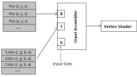
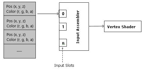
However, most of the time we will bind a single buffer of heterogeneous (various, mixed) attributes for all vertices: the whole vertex buffer.
Separated buffers of homogeneous attributes are useful if you need to only access some of the attributes. In that case, you can get better cache and bandwidth performance with separated buffers of homogeneous attributes, which allows cache lines and registers to only fetch the relevant data. Anyway, we don’t need to worry about these low-level details right now.
5.3 - Input layout
The input layout holds part of the state of the input assembler. In particular, it describes the vertex layout to let the input assembler know how to access the vertex attributes. Also, the input layout specifies, for each vertex attribute, the semantic name (to identify the attribute), a semantic index (to append to the semantic name in case there were more attributes with the same semantic name; that is, to distinguish them from each other), the format, the input slot, the offset (in bytes) from the start of the vertex, and other information. That way, the input assembler knows how to convey vertex attributes to the vertex shader through input registers (more on this shortly).
5.4 - Primitive topologies
In order to assemble primitives, the input assembler needs to know their basic type (point, line, triangle or patch) and topology, which allows to define a relationship between the primitives defined in a vertex buffer (connection, adiacency, and so on). We must provide this information, along with other details, to ensure that the input assembler properly interprets the vertex buffer data. The following image shows the main primitive types that the input assembler can generate from the vertex buffer data.
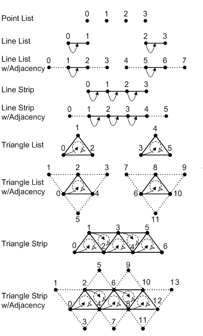
Point List indicates a collection of vertices that are rendered as isolated points. The order of the vertices in the vertex buffer is not important as it describes a set of separated points.
Line List indicates a collection of line segments. The two vertices that represent the extremes of each line segment must be contiguous in the vertex buffer.
Line Strip indicates a connected series of line segments. In the vertex buffer, the vertices are ordered so that the first vertex represents the starting point of the first segment of the line strip, the second vertex represents both the end point of the first segment and the starting point of the second segment, and so on.
Triangle List indicates a series of triangles that make up a mesh. The three vertices of each triangle must be contiguous in the vertex buffer, and in a specific order (clockwise or counterclockwise).
Triangle Strip indicates a series of connected triangles that make up a mesh. The three vertices of the i-th triangle in the strip can be determined according to the formula $\triangle_i=\{i,\quad i+(1+i\%2),\quad i+(2-i\% 2)\}$.
As you can see in the image above, this allows to have an invariant winding order (clockwise or counterclockwise) of the vertices of each triangle in the strip.
Adjacent primitives are intended to provide more information about a geometry and are only visible through a geometry shader. We will return to adjacent primitives in a later tutorial.
5.5 Index buffer
Consider the following figure.
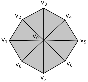
Here, we have a geometry composed of 8 primitives (triangles) and 9 vertices. However, the vertex buffer that describes this geometry as a triangle list contains 24 vertices with lots of repetitions.
Vertex octagon[24] = {
v0, v1, v2, // Triangle 0
v0, v2, v3, // Triangle 1
v0, v3, v4, // Triangle 2
v0, v4, v5, // Triangle 3
v0, v5, v6, // Triangle 4
v0, v6, v7, // Triangle 5
v0, v7, v8, // Triangle 6
v0, v8, v1  // Triangle 7
};
To avoid duplication in the vertex buffer, we can build an index buffer that describes the geometry as a triangle list by picking up vertices in the vertex buffer. For example,
Vertex v[9] = { v0, v1, v2, v3, v4, v5, v6, v7, v8 };

UINT indexList[24] = {
0, 1, 2, // Triangle 0
0, 2, 3, // Triangle 1
0, 3, 4, // Triangle 2
0, 4, 5, // Triangle 3
0, 5, 6, // Triangle 4
0, 6, 7, // Triangle 5
0, 7, 8, // Triangle 6
0, 8, 1  // Triangle 7
};
Now, the vertex buffer only contains 9 vertices. Although we have repeated some vertices in the index buffer, it’s important to note that indices are usually stored as short integers (2 bytes), whereas vertices are complex structures that require more memory to be stored. Using an index buffer can help save memory space. However, since the vertex buffer used in this tutorial only contains 3 vertices to describe a triangle, we will not be using an index buffer. Anyway, an index buffer can be bound to the command buffer just like a vertex buffer. However, unlike a vertex buffer, it doesn’t require any additional information to be bound to the pipeline since it only contains integer values (that is, the input assembler knows how to interpret the data from an index buffer).
5.6 - System-Generated Values
In addition to the vertex attributes from the vertex buffer, the input assembler can also pass to the next stages some system-generated values, such as a primitive ID and/or a vertex ID. These values assist subsequent stages in identifying the primitives generated and the vertices processed by the input assembler.
6 - The Vertex Shader
The vertex shader processes, one by one, the vertices of the primitives generated by the input assembler. For this purpose, the input assembler outputs vertex attributes to input variables declared in the vertex shader code. These input variables are associated with vertex attributes by using the same semantic names applied to vertex attributes in the input layout (as explained in section 5.3).
Typically, the vertex shader is responsible for transforming vertices to scale, rotate, or translate a mesh before passing the results to the next stage through output variables, which of course become input variables in that stage.
[!NOTE]
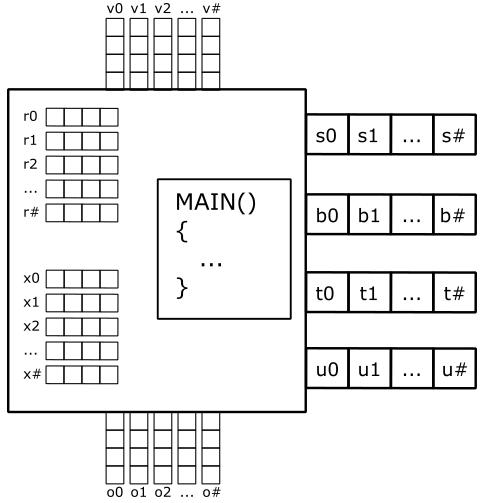
The image below shows a simplified design of a shader core, as exposed by the shader model, which abstract\hide the hardware details to expose the rendering pipeline to the programmer.
Binding slots (s#, b#, t# and u#) are used to associate resources in memory with variable declarations in the shader code, as discussed in section 3.4.
128-bit registers are used for input and output data (v# and o#), and for temporary data (r# and x#). Each register can be seen as a four 32-bit component vector (that’s why you see arrays of four squares in the image above). For example, a vertex shader can receive the position of a vertex (from the input assembler) in the input register v0, and the color in the input register v1. Then, it can transform the position using a temporary register and put the result in the output register o0 to pass the data to the next stage. A shader core also provides shader registers (that are not shown in the illustration above) for constant buffer references (cb#), and input and output resource references (t# and u#). The symbol # is used because the number of registers of a certain type depends on the stage\shader type. In this context, a shader core is similar to a CPU core. However, unlike CPU programs, you will hardly write shader code in assembly language. Despite this, looking at the assembly code of shader programs is a crucial task in the optimization process to speed up the execution of your graphics applications. Observe that, as stated above, shader cores are just an abstraction of real hardware to “execute” bytecode instead of actual GPU instructions.
An important thing to understand is that GPUs have no idea what pipelines, stages, and shader cores are because they typically have hardware cores with 32-bit registers that execute the same instruction in parallel on scalar data within different threads. This is known as a SIMT (Single Instruction Multiple Threads) architecture. On the other hand, a rendering pipeline runs on shader cores, which provide an abstraction to enable a SIMD (Single Instruction Multiple Data) architecture. This means that each shader core can execute a single instruction on multiple (vector) data within a single thread. Also, a rendering pipeline is required a theoretical sequential processing of the primitives generated by the input assembler. However, in practice this restriction applies only when necessary. That is, a GPU can execute shaders in parallel on its cores for different primitives (in any order) until it needs to perform a task depending on the order of such primitives. We will return to these low-level details in later tutorials.
[!NOTE]
You may wonder why we stated in section 3.4 that there are no registers or memory regions behind binding slots (virtual register) despite the existence of cb# registers for constant buffers (CBVs) and t# registers for shader resource views (SRVs), for example. The essence of that statement is that there are no hardware registers or GPU memory space behind slots. Indeed, remember that shader registers only exist in the context of the shader model, which abstracts real hardware. So, at the end, a slot is just a name used by the GPU for linkage purposes to dispatch resource references or actual data to GPU core registers.
The listing below shows an example of a vertex shader. As you can see, input variables are explicitly declared as parameters of the entry point. However, you have the option to include them within a structure. The same applies to output variables. If you are passing a single variable to the next stage, you can explicitly declare it as the return value of the entry point. However, if multiple output variables are involved, you must use a structure encompassing all the output variables.
struct VSIntput
{
    float4 position : POSITION;
    float4 color : COLOR;
};

struct VSOutput
{
    // data to output to the next stage
};


// Explicitly declare the input vars as params of the entry point.
// Therefore, the VSIntput struct is useless in this case.
VSOutput VSMain(float4 position : POSITION, float4 color : COLOR)
{
    // Use position and color to output the data that the next stage expects as input
}

// Equivalent but use the VSIntput struct
// VSOutput VSMain( VSIntput )
// {
//     // use position and color to output data that the next stage expects as input
// }
If no optional stage is used between the vertex shader and the rasterizer, the vertex shader must also compute a 2D representation from the 3D vertex positions passed as input by the input assembler. The rasterizer requires this information that can be passed by the last pre-rasterizer programmable stage by associating the corresponding output variable with the system-value semantic SV_POSITION.
However, there’s no point in providing further details right now, as the sample examined in this tutorial will use a vertex buffer where the vertex positions are already in 2D and projected onto the projection window (more on this in the last section). Also, we don’t need to apply any transformations to the triangle we want to show on the screen. Therefore, the vertex shader used by the sample will operate as a simple pass-through. We will return to transformations and projections in later tutorials.
7 - The Rasterizer
The rasterizer takes vertices of 2D primitives (projected onto the projection window), and passes to the next stage the pixels covered by these 2D representations of the original 3D primitives. For this purpose, the rasterizer first use the viewport to transform the 2D vertex positions to render target positions, so that it can consider them with respect to the space of the render target. At that point, the rasterizer can compute the pixels covered by the 2D primitives so that to each pixel corresponds a texel in the render target at the same location. Then, it uses the scissor to discard the pixels falling outside a rectangular region on the render target. As you can see in the image below, the viewport is represented as a rectangle jut like a scissor, so that we can select a region on the render target where to restrict the drawing operations (more details on the viewport will be provided in a later tutorial). Therefore, the viewport can be seen as a transformation to map\stretch the projection window onto a particular rectangle of the render target. On the other hand, the scissor rectangle can be seen as a filter to discard pixels.
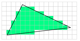
The calculation the rasterizer performs to check if a 2D primitive in the render target space covers a pixel is made with respect to itsl center. In other words, a pixel is covered if a primitive covers its center. Additionally, if two or more primitives overlap, the rasterizer generates and passes several pixels for the same texel position in the render target. However, which pixel is actually stored in the render target and how it is stored depends on whether blending, or depth and stencil tests are enabled. Additional details about this topics will be provided in a later tutorial, when we discuss the Output-Merger stage.
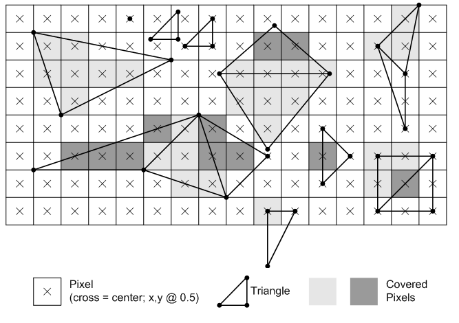
In the image above, light grey and dark grey colors are used for distinguishing between pixels generated for adjacent primitives. For example, in the top center of the figure, only two pixels (the dark grey ones) belong to the upper triangle. Despite the edge shared by the two triangles passes through the center of four pixels, the rasterizer can decide they belong to the lower triangle. Fortunately, we don’t need to know the rules that govern the rasterizer’s decisions. We usually just set the rasterizer state and enjoy the result in the pixel shader.
Behind the scene the rasterizer always passes to the pixel shader quads of $2\times 2$ pixels. Therefore, even if a single pixel of a quad is covered by a 2D primitive, the other pixels of the quad will be passed as well, as illustrated in the image below. The reason for this behavior will be explained in another tutorial. However, we can anticipate that all the pixels in a single quad will be processed by pixel shaders executed in parallel, and multiple quads of $2\times 2$ pixels can generally be processed in parallel.
![]()
It is worth mentioning that if a pixel is processed by a pixel shader but not covered by a primitive, it will be discarded when attempting to generate per-pixel data to write to the render target (which occurs when a value, such as a color, is returned by the pixel shader).
7.1 - Face culling
If specified in the rasterizer state stored (which is part of the PSO), the rasterizer can selectively pass to the next stage only pixels covered by front or back face triangles. This can optimize the rendering process by eliminating the rendering of faces that are not visible, reducing the number of polygons that need to be processed and rendered.
The front face of a triangle is the face that is oriented towards the normal vector. This vector is perpendicular to the triangle and points away from its front face. The rasterizer receives the vertices of each primitive in a specific order, specified in the input assembler state based on the primitive type and topology, and can determine whether a triangle is back-facing or front-facing by checking the sign of the triangle’s area computed in render target space. In a later tutorial, we will see how to derive a formula to compute the signed area of a triangle and how it can be used to establish whether a triangle is back-facing or front-facing.
The following image demonstrates the effect of setting the rasterizer state to cull the back face of triangles. In that case, the rasterizer will not generate any pixels for primitives showing their back face. This means that subsequent stages won’t process any pixels for those primitives, and you will see through them as if they were transparent.
7.2 - Attribute interpolation
We know that vertex attributes are data associated with vertices, but the rasterizer generates pixels from primitives. This raises a question: what color is a pixel inside a triangle? In other words, given the three vertices of a triangle storing color information, what is the color of a point within the triangle? Fortunately, the rasterizer can calculate this for us by interpolating the attributes of the vertices of a primitive using barycentric coordinates, and adjusting the result to account for the problems that arise when obtaining a 2D representation from a 3D primitive. Don’t worry if the last sentence seemed confusing. The rasterizer is a fixed-function stage, and we can simply welcome the result in the pixel shader without getting too caught up in the low-level details. However, the image below should help to illustrate why the rasterizer needs to fix the interpolation.
Consider an oblique line segment in 3D, defined by its two endpoints as vertices that hold both position and color attributes. If one vertex is black and the other is white, the center of the segment in 3D will appear gray. When this segment is projected onto the projection window, it will still appear as a line segment. However, if the rasterizer were to interpolate only the colors of the two projected endpoint vertices, the resulting gray pixel would be positioned at the center of the projected segment, rather than at the point where the center of the 3D segment is projected.
[!NOTE]
Interpolation also applies to depth values during the rasterization process. In other words, when the rasterizer generates pixels from primitives (e.g., triangles), it not only interpolates attributes like color, texture coordinates, and normals, but it also interpolates depth values.
8 - The Pixel shader
The pixel shader processes, one by one, the pixels sent by the rasterizer. It takes interpolated attributes as input (using registers v#) and produces per-pixel data as output (identified using the system-value semantic SV_Target), which can be stored in the render target at the corresponding position (i.e., at the corresponding texel in the render target). The pixel shader is typically used to compute per-pixel lighting and post-processing effects.
However, the sample examined in this tutorial does not implement per-pixel lighting or any special effects. Rather, it simply uses the interpolated color received by the rasterizer as the per-pixel data returned by the pixel shader.
[!NOTE]
We are only drawing a single triangle at the center of the window’s client area, which cannot be occluded by any other geometries or meshes. This means that the pixels generated by the rasterizer for this triangle will be the only ones processed by the pixel shader. Furthermore, we will not enable blending, depth testing, or stencil testing in the OM stage. As a result, most of the per-pixel data output by the pixel shader will definitely be stored in the render target, as the corresponding pixels will be covered by the triangle. Regarding the remaining pixels (the discarded ones), as we know, GPUs typically process quads of pixels in parallel. However, pixels that correspond to pixels not covered by primitives but still processed by the pixel shader will be discarded when attempting to generate per-pixel data to write to the render target. Therefore, in the case of our sample, the per-pixel data sent in output by the pixel shader for the pixels in a quad corresponding to pixels not covered by the triangle will be simply discarded.
[!NOTE]
If blending, depth testing, and stencil testing are disabled in the OM stage, per-pixel data returned by a pixel shader is always stored in the render target, unless the center of the corresponding pixel is not covered by a primitive, in which case the fragment is simply discarded by the fragment shader.
In this tutorial we won’t directly use the functionalities provided by the OM stage, except for setting the render target as the final output of the rendering pipeline. However, some blending information still needs to be defined in the PSO, at least to specify a bitmask controlling which components\channels of the texels in the render target can be written to (more on this in the next section).
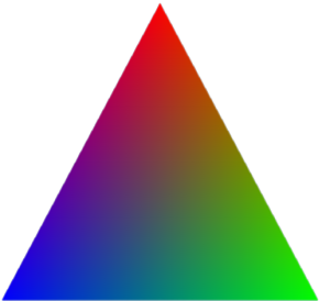
By running D3D12HelloTriangle, the sample examined in this tutorial, you can verify that the colors of the pixels inside the triangle, as well as those on its edges, are interpolated from the colors associated with the three vertices that describe the triangle in the vertex buffer.
9 - D3D12HelloTriangle: code review
We can finally review some code.
The application class now includes a root signature, a Pipeline State Object (PSO), a vertex buffer, and both viewport and scissor rectangles. It’s important to note that the comment regarding ComPtr highlights the necessity of not releasing COM objects on the CPU timeline before the GPU has finished using the corresponding resources on its timeline.
// Note that while ComPtr is used to manage the lifetime of resources on the CPU,
// it has no understanding of the lifetime of resources on the GPU. Apps must account
// for the GPU lifetime of resources to avoid destroying objects that may still be
// referenced by the GPU.
// An example of this can be found in the class method: OnDestroy().
using Microsoft::WRL::ComPtr;

class D3D12HelloTriangle : public DXSample
{
public:
    D3D12HelloTriangle(UINT width, UINT height, std::wstring name);

    virtual void OnInit();
    virtual void OnUpdate();
    virtual void OnRender();
    virtual void OnDestroy();

private:
    static const UINT FrameCount = 2;

    struct Vertex
    {
        XMFLOAT3 position;
        XMFLOAT4 color;
    };

    // Pipeline objects.
    CD3DX12_VIEWPORT m_viewport;
    CD3DX12_RECT m_scissorRect;
    ComPtr<IDXGISwapChain3> m_swapChain;
    ComPtr<ID3D12Device> m_device;
    ComPtr<ID3D12Resource> m_renderTargets[FrameCount];
    ComPtr<ID3D12CommandAllocator> m_commandAllocator;
    ComPtr<ID3D12CommandQueue> m_commandQueue;
    ComPtr<ID3D12RootSignature> m_rootSignature;
    ComPtr<ID3D12DescriptorHeap> m_rtvHeap;
    ComPtr<ID3D12PipelineState> m_pipelineState;
    ComPtr<ID3D12GraphicsCommandList> m_commandList;
    UINT m_rtvDescriptorSize;

    // App resources.
    ComPtr<ID3D12Resource> m_vertexBuffer;
    D3D12_VERTEX_BUFFER_VIEW m_vertexBufferView;

    // Synchronization objects.
    UINT m_frameIndex;
    HANDLE m_fenceEvent;
    ComPtr<ID3D12Fence> m_fence;
    UINT64 m_fenceValue;

    void LoadPipeline();
    void LoadAssets();
    void PopulateCommandList();
    void WaitForPreviousFrame();
};
As evident in the constructor of D3D12HelloTriangle (shown below), we will set the viewport and scissor rectangles to encompass the entire render target. This setup enables drawing on the entire back buffer (without stretching the image), while simultaneously discarding the pixels outside it (as they have no chance to be shown\mapped on the screen). Observe that, in Windows programming, a rectangle is often defined by specifying a starting point and a size.
D3D12HelloTriangle::D3D12HelloTriangle(UINT width, UINT height, std::wstring name) :
    DXSample(width, height, name),
    m_frameIndex(0),
    m_viewport(0.0f, 0.0f, static_cast<float>(width), static_cast<float>(height)),
    m_scissorRect(0, 0, static_cast<LONG>(width), static_cast<LONG>(height)),
    m_rtvDescriptorSize(0)
{
}
The code of the LoadPipeline function remains unchanged from the previous sample (D3D12HelloWindow). However, there are several additions in LoadAssets, so we will take the time to explain each one.
// Load the sample assets.
void D3D12HelloTriangle::LoadAssets()
{
    // Create an empty root signature.
    {
        CD3DX12_ROOT_SIGNATURE_DESC rootSignatureDesc;
        rootSignatureDesc.Init(0, nullptr, 0, nullptr, D3D12_ROOT_SIGNATURE_FLAG_ALLOW_INPUT_ASSEMBLER_INPUT_LAYOUT);

        ComPtr<ID3DBlob> signature;
        ComPtr<ID3DBlob> error;
        ThrowIfFailed(D3D12SerializeRootSignature(&rootSignatureDesc, D3D_ROOT_SIGNATURE_VERSION_1, &signature, &error));
        ThrowIfFailed(m_device->CreateRootSignature(0, signature->GetBufferPointer(), signature->GetBufferSize(), IID_PPV_ARGS(&m_rootSignature)));
    }

    // Create the pipeline state, which includes compiling and loading shaders.
    {
        ComPtr<ID3DBlob> vertexShader;
        ComPtr<ID3DBlob> pixelShader;

#if defined(_DEBUG)
        // Enable better shader debugging with the graphics debugging tools.
        UINT compileFlags = D3DCOMPILE_DEBUG | D3DCOMPILE_SKIP_OPTIMIZATION;
#else
        UINT compileFlags = 0;
#endif

        ThrowIfFailed(D3DCompileFromFile(GetAssetFullPath(L"shaders.hlsl").c_str(), nullptr, nullptr, "VSMain", "vs_5_0", compileFlags, 0, &vertexShader, nullptr));
        ThrowIfFailed(D3DCompileFromFile(GetAssetFullPath(L"shaders.hlsl").c_str(), nullptr, nullptr, "PSMain", "ps_5_0", compileFlags, 0, &pixelShader, nullptr));

        // Define the vertex input layout.
        D3D12_INPUT_ELEMENT_DESC inputElementDescs[] =
        {
            { "POSITION", 0, DXGI_FORMAT_R32G32B32_FLOAT, 0, 0, D3D12_INPUT_CLASSIFICATION_PER_VERTEX_DATA, 0 },
            { "COLOR", 0, DXGI_FORMAT_R32G32B32A32_FLOAT, 0, 12, D3D12_INPUT_CLASSIFICATION_PER_VERTEX_DATA, 0 }
        };

        // Describe and create the graphics pipeline state object (PSO).
        D3D12_GRAPHICS_PIPELINE_STATE_DESC psoDesc = {};
        psoDesc.InputLayout = { inputElementDescs, _countof(inputElementDescs) };
        psoDesc.pRootSignature = m_rootSignature.Get();
        psoDesc.VS = CD3DX12_SHADER_BYTECODE(vertexShader.Get());
        psoDesc.PS = CD3DX12_SHADER_BYTECODE(pixelShader.Get());
        psoDesc.RasterizerState = CD3DX12_RASTERIZER_DESC(D3D12_DEFAULT);
        psoDesc.BlendState = CD3DX12_BLEND_DESC(D3D12_DEFAULT);
        psoDesc.DepthStencilState.DepthEnable = FALSE;
        psoDesc.DepthStencilState.StencilEnable = FALSE;
        psoDesc.SampleMask = UINT_MAX;
        psoDesc.PrimitiveTopologyType = D3D12_PRIMITIVE_TOPOLOGY_TYPE_TRIANGLE;
        psoDesc.NumRenderTargets = 1;
        psoDesc.RTVFormats[0] = DXGI_FORMAT_R8G8B8A8_UNORM;
        psoDesc.SampleDesc.Count = 1;
        ThrowIfFailed(m_device->CreateGraphicsPipelineState(&psoDesc, IID_PPV_ARGS(&m_pipelineState)));
    }

    // Create the command list.
    ThrowIfFailed(m_device->CreateCommandList(0, D3D12_COMMAND_LIST_TYPE_DIRECT, m_commandAllocator.Get(), m_pipelineState.Get(), IID_PPV_ARGS(&m_commandList)));

    // Command lists are created in the recording state, but there is nothing
    // to record yet. The main loop expects it to be closed, so close it now.
    ThrowIfFailed(m_commandList->Close());

    // Create the vertex buffer.
    {
        // Define the geometry for a triangle.
        Vertex triangleVertices[] =
        {
            { { 0.0f, 0.25f * m_aspectRatio, 0.0f }, { 1.0f, 0.0f, 0.0f, 1.0f } },
            { { 0.25f, -0.25f * m_aspectRatio, 0.0f }, { 0.0f, 1.0f, 0.0f, 1.0f } },
            { { -0.25f, -0.25f * m_aspectRatio, 0.0f }, { 0.0f, 0.0f, 1.0f, 1.0f } }
        };

        const UINT vertexBufferSize = sizeof(triangleVertices);

        // Note: using upload heaps to transfer static data like vert buffers is not
        // recommended. Every time the GPU needs it, the upload heap will be marshalled
        // over. Please read up on Default Heap usage. An upload heap is used here for
        // code simplicity and because there are very few verts to actually transfer.
        ThrowIfFailed(m_device->CreateCommittedResource(
            &CD3DX12_HEAP_PROPERTIES(D3D12_HEAP_TYPE_UPLOAD),
            D3D12_HEAP_FLAG_NONE,
            &CD3DX12_RESOURCE_DESC::Buffer(vertexBufferSize),
            D3D12_RESOURCE_STATE_GENERIC_READ,
            nullptr,
            IID_PPV_ARGS(&m_vertexBuffer)));

        // Copy the triangle data to the vertex buffer.
        UINT8* pVertexDataBegin;
        CD3DX12_RANGE readRange(0, 0);        // We do not intend to read from this resource on the CPU.
        ThrowIfFailed(m_vertexBuffer->Map(0, &readRange, reinterpret_cast<void**>(&pVertexDataBegin)));
        memcpy(pVertexDataBegin, triangleVertices, sizeof(triangleVertices));
        m_vertexBuffer->Unmap(0, nullptr);

        // Initialize the vertex buffer view.
        m_vertexBufferView.BufferLocation = m_vertexBuffer->GetGPUVirtualAddress();
        m_vertexBufferView.StrideInBytes = sizeof(Vertex);
        m_vertexBufferView.SizeInBytes = vertexBufferSize;
    }

    // Create synchronization objects and wait until assets have been uploaded to the GPU.
    {
        ThrowIfFailed(m_device->CreateFence(0, D3D12_FENCE_FLAG_NONE, IID_PPV_ARGS(&m_fence)));
        m_fenceValue = 1;

        // Create an event handle to use for frame synchronization.
        m_fenceEvent = CreateEvent(nullptr, FALSE, FALSE, nullptr);
        if (m_fenceEvent == nullptr)
        {
            ThrowIfFailed(HRESULT_FROM_WIN32(GetLastError()));
        }

        // Wait for the command list to execute; we are reusing the same command
        // list in our main loop but for now, we just want to wait for setup to
        // complete before continuing.
        WaitForPreviousFrame();
    }
}
First, we create an empty root signature (with no root parameters and static samplers) as the shader programs used by this sample don’t need to access any GPU memory resources (we will review the shader code at the end of the tutorial). We use the CD3DX12_ROOT_SIGNATURE_DESC structure, and its Init helper function, to specify root parameters, static samplers and flags.
The flag D3D12_ROOT_SIGNATURE_FLAG_ALLOW_INPUT_ASSEMBLER_INPUT_LAYOUT specifies we want to use the input assembler as a stage of the pipeline (indeed, we can also render without it, but we won’t cover the details here as it goes beyond the scope of this tutorial). On some GPUs, omitting this flag can save an additional DWORD in the root argument space to store our root arguments. Omit this flag if the input assembler is not required, though the optimization is minor.
We create a serialized version of the root signature by calling D3D12SerializeRootSignature. This generates a memory blob of the root signature, which can then be used to create the root signature object using the CreateRootSignature function. The serialized version could be stored in a file on disk for quick loading, eliminating the need to recreate it each time. To store the serialized version in memory we use a pointer to a ID3DBlob interface. This interface is used to hold generic byte arrays called memory blob (whether it be object code or a simple vertex array; it’s up to the programmer to cast data to the correct type) that can be easily stored to disk using the D3DWriteBlobToFile function.
Root signatures can also be defined directly within shader code. In such cases, the shader code and the root signature are compiled together into the same memory blob.
For the current sample, we employ the root signature version 1.0, as specified by the second argument passed to D3D12SerializeRootSignature. In subsequent tutorials, we will switch to version 1.1. As a general rule, it’s always advisable to use the most recent root signature version unless you have a valid reason to use an older version.
Then, we compile the shaders with D3DcompileFromFile to get the bytecode of each shader program as a memory blob. In this case, we are using a vertex shader and a pixel shader as the only two programmable stages of the rendering pipeline to render a triangle on the screen. The D3DcompileFromFile function takes the path to the file containing the shader code (written in HLSL language), the entry point of the program, a shader target (specified as a string), some flags (as a bit field), and the address of the ID3DBlob interface pointer that the function will use to store the bytecode. It’s worth noting that you can have the code for multiple shaders (e.g., both vertex and pixel shaders) stored in a single file on disk.
[!NOTE]
Typically, a shader target is a string that identifies a specific shader model. The High-Level Shading Language (HLSL) is employed to program in the context of a shader model, which defines the architecture and capabilities of the shader cores and exposes the rendering pipeline to the programmer. Each shader model builds on the capabilities of the model before it, implementing more functionality with fewer restrictions. Consequently, by utilizing the latest shader models, developers can write more feature-rich shader programs in HLSL.
As mentioned earlier, the input layout is used to define part of the input assembler state. In this case, we specify that each vertex in the vertex buffer has two elements\attributes: a position and a color. POSITION and COLOR are the string used as semantic names in the input layout, allowing the vertex shader to use the corresponding attributes through the input variables marked with the same semantic names (we will review the shader code at the end of the tutorial). Since we don’t have multiple attributes using the same semantic name, the semantic index is set to zero for both position and color. The format of the position attribute is an array of three 32-bit floating-point values (representing the x-, y-, and z-coordinates), while the format of the color attribute is an array of four 32-bit floats to store the corresponding RGBA values.
We have a single vertex buffer that contains the three vertices describing a triangle (i.e., we won’t use separate vertex buffers for each attribute), so we set zero as the binding slot for both position and color attributes. We set zero as byte offset from the start of the vertex structure for the position attribute, which is the first one. On the other hand, we set 12 for the byte offset of the second attribute (the color) as it follows the position attribute, which is an array of 3 floats (a float is a 4 bytes, so 3 * 4 = 12). D3D12_INPUT_CLASSIFICATION_PER_VERTEX_DATA specifies the attribute is per-vertex data.
[!NOTE]
On the other hand, D3D12_INPUT_CLASSIFICATION_PER_INSTANCE_DATA specifies that the attribute is per-instance data. Indeed, you can draw more instances of the same mesh\geometry with a single draw command, in which case the last field of the correspondingD3D12_INPUT_ELEMENT_DESC structure specifies the number of instances to draw using the same per-instance data before advancing in the per-instance buffer by one element. We’ll cover instancing in a later tutorial.
Then, we create a PSO with CreateGraphicsPipelineState.
In addition to the input layout just created, we specify that a triangle will be used as the basic type to describe primitives in the vertex buffer. Together, these two pieces of information don’t cover the whole input assembler state, though. We still need to set the topology in the command list (more on this shortly).
We also set the root signature, the bytecode (for vertex and pixel shaders) and the format of the render target (sometimes it can be different from the format of the buffers in the swap chain; for example, when you want to draw on a different texture in order to implement some off-screen rendering techniques).
We set a default blend state, which disable blending, while enabling writing to all components\channels of the texels in the render target. This means that the per-pixel data returned by a pixel shader won’t be blended with the corresponding texel data in the render target but will simply be stored as it is.
Also, we disable depth and stencil tests as we have a single triangle that can’t be occluded. Blending information, depth and stencil tests, and the specification of a render target are all part of the output-merger stage, which will be covered in more detail in a later tutorial.
We set a default state for the rasterizer stage as well. This indicates we are interested in pixels covered only by front-face triangles, whose vertices are in clockwise order.
D3D12_GRAPHICS_PIPELINE_STATE_DESC::SampleMask is a bitmask controlling which samples are used to generate a final pixel during multisampling. Although we won’t use multiple samples per pixel for a while, we’ll still set it to 0xFFFFFFFF, indicating all of them, regardless of their number.
During the creation of a command list, we can pass a PSO as an argument to set the pipeline state. In this case, we pass the PSO just created as an argument to CreateCommandList.
To create the vertex buffer, we first use the Vertex structure defined in the application class to build an array of vertices. Ineed, in this case, the vertex buffer is an array of only 3 vertices specified in clockwise order, with position and color as vertex attributes (in accordance with the input layout). As you may notice, the last coordinate of the position (the z-coordinate) is $0.0$ for all three vertices. This means the triangle lies in the XY-plane, where also lies the projection window. This presents a significant advantage as we already have a 2D representation of the triangle, and we only need to ensure that it is within the projection window’s boundaries.
[!NOTE]
In a later tutorial we will see that a projected primitive is inside the 2D projection window (in front of the camera) as long as the x- and y-coordinates of its vertex positions are in the range $[−1,\ 1]$, while the z-coordinate is in the range $[0,\ 1]$. As you can see in the definition of the array of vertices, that’s exactly the case of our triangle, which will be rendered for sure.
Once the array of vertices is ready, we must transfer it to a GPU heap for use as a vertex buffer by the input assembler. ID3D12Device::CreateCommittedResource serves a dual purpose, creating a resource while also allocating sufficient GPU heap memory space to accommodate the entire resource. As discussed earlier, there are three types of GPU heaps where memory space can be allocated:
-
D3D12_HEAP_TYPE_DEFAULT specifies the default heap. This heap type experiences the most bandwidth for the GPU, but cannot provide CPU access.
-
D3D12_HEAP_TYPE_UPLOAD specifies the upload heap. This heap type has CPU access optimized for write operations, but might not experience the maximum amount of bandwidth for the GPU. Resources in this heap must be created with D3D12_RESOURCE_STATE_GENERIC_READ and cannot be changed away from this. Typical usages for upload heaps are:
- Initializing resources in a default heap with data from the CPU.
- Uploading dynamic data in a constant buffer that is read, repeatedly, for each vertex or pixel.
-
D3D12_HEAP_TYPE_READBACK Specifies the readback heap. This heap type has CPU access optimized for reading data back from the CPU, but does not experience the maximum amount of bandwidth for the GPU.
-
D3D12_HEAP_TYPE_CUSTOM Specifies a custom heap. The application may specify the memory pool and CPU cache properties directly. To do so, the application is expected to understand the adapter architecture to make the right choice.
Based on the definitions above, we should allocate memory space on the upload heap to write the vertex array from our application, and then use that memory space to initialize memory allocated on the default heap for use as the vertex buffer. This approach is recommended because, once the vertex buffer is initialized, we no longer need to access it from the CPU to modify the vertices (in this case, the vertex buffer is considered static). However, for the sake of simplicity, in this sample we will directly employ the vertex array in the upload heap as the vertex buffer. This means the GPU might access the vertex buffer through the PCI-e bus, which is slower. We will explore the use of other heaps in later tutorials.
ID3D12Resource::Map maps a GPU resource to the virtual address space of our C++ (CPU) application. It returns (as an output parameter) a pointer to the CPU-visible GPU heap memory where the resource is stored (so it only works for resources stored on upload and readback heaps).
In Direct3D, resource access occurs at a subresource granularity. In other words, a subresource is the smallest resource we can access in memory, except for tiled resources (which we will delve into in later tutorials). In this case, we use zero as an argument for the first parameter of Map to indicate that we want to map the entire vertex buffer — a simple resource with no subresources or a single subresource encompassing the entire resource; either interpretation is valid. Map also takes a pointer to a D3D12_RANGE structure as a parameter that describes the region of memory that the CPU might read. Since the resource is stored in the upload heap, which is write-combine memory, we shouldn’t read it from the CPU. Therefore, we initialize the range to $[0,\ 0]$ to specify that the CPU won’t read any data from the mapped resource (passing a null pointer instead would indicate the entire resource). The last parameter of Map is a pointer to a memory block that will receive the CPU virtual address of the mapped resource, as mentioned earlier.
[!NOTE]
The pointer returned in the last parameter is never offset by any values in the D3D12_RANGE structure. This means that ID3D12Resource::Map always maps starting from the beginning of the specified subresource for writing purposes.
We use memcpy to copy the array of vertices to the CPU-mapped version of the vertex buffer (recall that we can do this as the upload heap is accessible by the CPU). Then, we invoke ID3D12Resource::Unmap to unmap the vertex buffer from the virtual address space of our application (as we don’t need it anymore).
[!NOTE]
Observe that to create a vertex buffer view, we need the address and size of the vertex buffer, as well as the size in bytes of each vertex (StrideInBytes field) to inform the input assembler when it is accessing a new vertex\entry in the vertex buffer. Remember that vertex buffer views are not stored in descriptors as they are recorded in (copied to) a command list when we want to bind them to the input assembler.
Lastly, we create a fence and call WaitForPreviousFrame at the end of LoadAssets. However, we don’t really need it here, as there is nothing in the command list right now. We will revisit this concept in a later tutorial.
Now, we can review the code of PopulateCommandList.
void D3D12HelloTriangle::PopulateCommandList()
{
    // Command list allocators can only be reset when the associated
    // command lists have finished execution on the GPU; apps should use
    // fences to determine GPU execution progress.
    ThrowIfFailed(m_commandAllocator->Reset());

    // However, when ExecuteCommandList() is called on a particular command
    // list, that command list can then be reset at any time and must be before
    // re-recording.
    ThrowIfFailed(m_commandList->Reset(m_commandAllocator.Get(), m_pipelineState.Get()));

    // Set necessary state.
    m_commandList->SetGraphicsRootSignature(m_rootSignature.Get());
    m_commandList->RSSetViewports(1, &m_viewport);
    m_commandList->RSSetScissorRects(1, &m_scissorRect);

    // Indicate that the back buffer will be used as a render target.
    m_commandList->ResourceBarrier(1, &CD3DX12_RESOURCE_BARRIER::Transition(m_renderTargets[m_frameIndex].Get(), D3D12_RESOURCE_STATE_PRESENT, D3D12_RESOURCE_STATE_RENDER_TARGET));

    CD3DX12_CPU_DESCRIPTOR_HANDLE rtvHandle(m_rtvHeap->GetCPUDescriptorHandleForHeapStart(), m_frameIndex, m_rtvDescriptorSize);
    m_commandList->OMSetRenderTargets(1, &rtvHandle, FALSE, nullptr);

    // Record commands.
    const float clearColor[] = { 0.0f, 0.2f, 0.4f, 1.0f };
    m_commandList->ClearRenderTargetView(rtvHandle, clearColor, 0, nullptr);
    m_commandList->IASetPrimitiveTopology(D3D_PRIMITIVE_TOPOLOGY_TRIANGLELIST);
    m_commandList->IASetVertexBuffers(0, 1, &m_vertexBufferView);
    m_commandList->DrawInstanced(3, 1, 0, 0);

    // Indicate that the back buffer will now be used to present.
    m_commandList->ResourceBarrier(1, &CD3DX12_RESOURCE_BARRIER::Transition(m_renderTargets[m_frameIndex].Get(), D3D12_RESOURCE_STATE_RENDER_TARGET, D3D12_RESOURCE_STATE_PRESENT));

    ThrowIfFailed(m_commandList->Close());
}
In resetting the command list, we pass the PSO as an argument to set the pipeline state. Remember that if you pass a null pointer, a default pipeline state will be set, and we want to prevent this behavior as we have a custom PSO to set.
Next, we associate the root signature with the command list using SetGraphicsRootSignature to set up the parameter space.
We need to record some commands in the command list to set the pipeline states outside the PSO.
To complete the input assembler state, we bind the vertex buffer view using IASetVertexBuffers and set the topology with IASetPrimitiveTopology. In this case, we set TRIANGLELIST as we have a single triangle described with 3 contiguous vertices in the vertex buffer, in clockwise order.
The rasterizer state is completed by setting the viewport and scissor rectangles, which are the same size as the render target so that we can draw on the whole back buffer.
To complete the output-merger state, we call OMSetRenderTargets, which binds the current render target as the final output of the rendering pipeline.
[!NOTE]
Some rendering techniques require writing different per-pixel data to different render targets. To avoid restarting the rendering pipeline each time we need to write to a different render target, Direct3D allows writing to multiple render targets simultaneously (we can select the render target to store a value with SV_Target[n], where n is the index of the render target). This is why OMSetRenderTargets takes the number of render targets as the first parameter and an array of render targets as the second parameter. It also explains why we need to pass arrays of viewport and scissor rectangles to RSSetViewports and RSSetScissorRects, respectively.
The third parameter of OMSetRenderTargets is a boolean that specifies whether the handle passed as an argument to the second parameter is a pointer to a contiguous range of RTVs in a descriptor heap. In this case, we pass FALSE, indicating that the handle is the first of an array of handles to descriptors. In our case, it’s okay to pass FALSE, as we only have a handle to the RTV we want to bind. We will delve into these advanced topics in later tutorials.
ID3D12GraphicsCommandList::DrawInstanced instructs the GPU to draw one or more instances of a mesh. In this case, we will draw a single triangle. When the GPU executes this command, the rendering pipeline starts working. The first parameter of DrawInstanced is the number of vertices to draw per instance (that is, it is the number of vertices that make up the primitives of the mesh in the vertex buffer, so it’s also the number of times the vertex shader will be executed per instance; remember that the vertex shader processes the primitives one vertex at a time). The remaining parameters will be explained in a later tutorial.
To conclude this section, let’s take a look at the shader code.
struct PSInput
{
    float4 position : SV_POSITION;
    float4 color : COLOR;
};


PSInput VSMain(float4 position : POSITION, float4 color : COLOR)
{
    PSInput result;

    result.position = position;
    result.color = color;

    return result;
}


float4 PSMain(PSInput input) : SV_TARGET
{
    return input.color;
}
The PSInput structure declares both the output of the vertex shader and the (interpolated) input the pixel shader expects from the rasterizer. It is possible to have a single structure for both shaders as the per-pixel attributes are a simple interpolation of the per-vertex attributes (that is, we have the same type and number of attributes both per-vertex and per-pixel).
The system-value semantic SV_POSITION identifies a special position both in the output of the vertex shader and in the input of the pixel shader. In the context of a vertex shader, this semantic specifies the 2D representation of a 3D vertex position (recall that the rasterizer expects a 2D representation of 3D primitives). In the context of a pixel shader, SV_POSITION specifies the pixel position of the pixel currently processed (offset by 0.5 to get the position of its center). In other words, it identifies the render target coordinates of the pixel; remember that the pixel shader processes pixels related to texels in the render target, so the rasterizer can easily compute this value. However, the pixel position is rarely used in the pixel shader unless you need to implement some advanced rendering techniques.
The semantic COLOR is used to simply convey the color attribute of the vertices from the input assembler (remember how we built the vertex buffer and set up the input layout) up to the pixel shader, where it is returned as the per-pixel data to store in the render target (at the same position of the currently processed pixel).
[!NOTE]
You may wonder why we need to use a float4 to describe a position in the PSInput structure if we defined it as an array of three floats in the vertex buffer (for the x-, y- and z-coordinates). Actually, you can use a float3 as the first input parameter (position) for the entry point of the vertex shader. However, you can’t change the type of the position field in the PSInput structure. We will see why in an upcoming tutorial.
The vertex shader specified within the PSO is executed for each vertex of the primitives generated by the input assembler. In this case, we have a vertex buffer containing just three vertices (red, green, and blue) that represent a single triangle. Therefore, the vertex shader runs three times (almost certainly in parallel). The vertex shader can perform a wide range of tasks, but it is typically used to obtain a sort of 2D representation of the 3D primitives that constitute the meshes in a 3D scene. Actually, we already have a 2D representation of the triangle we wish to render on the screen, so we’ll use the vertex shader as a straightforward pass-through to transfer data from the input assembler to the rasterizer. In accordance with the input layout, the entry point of the vertex shader is VSMain. The input layout also defines the semantics employed to transmit the vertex attributes so, in the vertex shader, we associate the same semantics to the input parameters of VSMain to indicate where we want to receive the corresponding attributes from the input assembler. Observe that we might have also defined a VSInput structure to pass position and color as parameters to VSMain, similar to how we pass a PSInput structure to PSMain.
The rasterizer identifies the pixels occupied by the projected, 2D primitives (passed by the last pre-rasterizer shader through the SV_POSITION semantic) and then interpolates output vertex attributes (in this case color and position) for those pixels in order to convey the result to the pixel shader. Pixels covered by primitives outside the projection window are discarded to prevent the pixel shader from wasting time processing pixels that won’t be displayed on the screen. Remember that, in this case, the viewport and scissor are the same size as the render target, ensuring that the triangle will be rendered across the entire back buffer.
The pixel shader processes, one by one, the pixels covered by the projected, 2D primitives processed by the rasterizer. In this case, we don’t need to perform any specific tasks or tests in the pixel shader, so we simply return the interpolated color as the per-pixel data to store in the render target at the corresponding position (that is, in the texel associated with the currently processed pixel). If you run the sample, you will notice that the colors of the pixels inside the triangle, and along its edges, are interpolated from the colors associated with the three vertices in the vertex buffer. Remember that the system-value semantic SV_TARGET is used to identify the output value returned by the pixel shader as the per-pixel data that could be stored in the render target. When you have a pixel shader that return a single value as the per-pixel data, you can specify SV_TARGET for that value after the pixel shader’s entry point, followed by a colon symbol. In this case, the per-pixel data will be stored for sure as we haven’t enabled blending, depth or stencil testing in the output merger stage.
[!NOTE]
Execute the sample and try resizing the window. What happens? The triangle gets stretched because we have a swap chain with two buffers of $1280\times 720$, while the window no longer matches the same size. You can mitigate the problem by resizing the window to a dimension with an aspect ratio similar to $1280/720$. However, we will ultimately fix this problem in a later tutorial.
Source code: D3D12HelloWorld (DirectX-Graphics-Samples)
References
[1] DirectX graphics and gaming (Microsoft Docs)
[2] DirectX-Specs (Microsoft Docs)
If you found the content of this tutorial somewhat useful or interesting, please consider supporting this project by clicking on the Sponsor button. Whether a small tip, a one time donation, or a recurring payment, it’s all welcome! Thank you!
